Fundamentals of Data Analytics (32130) Week 3

CRISP-DM

6 phases, but not every project requires all 6.

Business understanding

The first stage in the CRISP-DM methodology is crucial in any data mining project, and emphasises understanding the objectives of the relevant project in its business context and then strategically achieving those objectives. Explained below are the four steps in the business understanding stage.

Determine the business objectives

it is equally critical to understand the business problem or question which a client wants to achieve in a particular project. Therefore, the data specialist shall need to rigorously understand and identify specific business issues for solving them with authenticity. Also, the data expert needs to set the scope of the project to successfully meet its objectives.

Assess the situation

the data analyst sets the projection for the resources (i.e. required human resources and tools) required to undertake the data mining project in this step. Moreover, experts must uncover the available data to attain the primary business objective. They should also outline the project risks, their solutions and develop a cost-benefit analysis for the project.

Determine the data mining goals

the data mining goal should be crafted so that it can be quantitatively assessed and predicted with accuracy. For instance, predicting sales in a market based on historical data analysis including past purchases and user demographics. It will be advisable to tweak the problem itself in case of failure to effectively translate the business goal into a data mining goal.

Produce a project plan

in this step, a thorough project plan is developed to demonstrate the potential method for reaching the data mining goals. The plan includes specifying steps/stages, a proposed timeline, an assessment of potential risks and an initial assessment of the tools and techniques required to facilitate the project.

Data understanding

the exploration stage where an expert looks for ways to understand more about the data usefulness, data quality, initial insights from data for finding interesting subsets to develop hypotheses about uncovered information. Initial facts and figures collection is done from all available sources. Then the properties of the data acquired are examined. The quality of the information is then verified by answering certain relevant questions concerning the completeness and accuracy of the material. The four steps in this stage are explained below.

Collect the initial data

the data expert collects the required data and ensures the prior reporting of any problems that might occur due to a multisource data gathering process that may cause time lags and can delay the project.

Describe the data

in this step, the analyst identifies superficial findings about the data including data format, data quantity, the number of records and the fields in each table, the identities of the fields, and any other surface features of the data. This step is an initial milestone leading to the upcoming steps, provided that the collected data meets the project requirements.

Explore the data

visualisations or reports can be generated to develop some initial data patterns which then can be used for exploring the prospective impacts on the rest of the project.

Verify data quality

the data expert assesses the data quality by cross-checking different variables, missing values or attributes and the authenticity of values.

Data preparation

This stage involves various data organisation activities including tables, records, and attribute selection, transformation and cleaning of data. The process helps in extracting the final data set and to make it ready for modelling tools. Exploration of information may be executed for finding patterns in light of business understandings. There are five steps in the data preparation stage.

Select data

in this process, decisions about data selection are made – what pieces of data are needed and do they meet with the data mining goals? It is also important to clearly justify the need for the use of some attributes over others that might be less useful in the project.

Clean data

this step is relevant to the assessment of data quality and cleansing. It is a crucial process as it will decide the final project outcomes. Modelling analyses can be used to estimate the missing data for assuring project data quality.

Construct data

creating or extracting new attributes from existing ones could help in easing the data analysis process. This step should be used by experts to carefully add new or derived attributes for simplifying the modelling process. New attributes may include the conversion of symbols or words into numeric values which in most cases are required by tools or algorithms.

Integrate data

this process helps in integrating or combining data from different tables or records into a single entity or table. The analyst can do this by combining information to be summarised from multiple tables of the same object.

Format data

it is required in certain cases that the data expert should change the format or design of the data to meet the requirements of modelling tool(s), or in other cases, the data modification is crucial to project the right data mining question.

Modelling

A number of modelling methods are used to solve the data mining problem, and their parameters are adjusted accordingly. Different techniques/methods can be applicable to one data problem, though some methods are only suitable for particular forms of data sets. The essential steps are explained below.

Select the modelling technique

this step is related to the selection of modelling techniques based on the assumptions each technique makes.

Generate test design

it is essential for a data expert to test and validate the model quality by conducting experiments. These experiments will demonstrate how well the proposed model/technique fits the problem, and will prepare a base for gradual model improvements.

Build the model

the selected modelling tool is used in this stage to run the refined data set for developing single or a range of models.

Assess the model

in this stage, the data analyst makes inferences about the data based on his/her domain knowledge and produces the results which in some cases cannot be generalised. It is therefore suggested that the analyst should work with multi domain experts to showcase the results in different contexts. To do so, the analyst evaluates the project criteria by considering wide objectives and iteratively using multiple modelling techniques to discover different inferences.

Evaluation

It is very important for the data expert to rigorously evaluate the model and the attainment of project objectives before its final placement. After going through the following steps, the project team will be able to use the outcomes as per their requirements.

Evaluate results

this process is intense in examining the quality and applicability of the model in achieving the original business objectives. It is also explored here if there are any gaps in the model that could have an impact on future outcomes. Also, a completion statement is developed by a data analyst.

Review process

a thorough review is done in this step to look for any important factors that might have been overlooked by the analyst while developing the model and that can possibly hinder future model deployments.

Determine next steps

the project leader at this stage decides to execute the project if no new data mining projects are considered.

Deployment

The development of the model on its own is not the closure of project, but the inferences or insights derived from the data model should be translated into end-user applications including online/web interfaces, marketing materials and personalised devices. The deployment stage varies with varying users and their on-demand requirements. For a user, it can be as simple as developing a basic report to developing a big database for any other complex projects. The following steps are the ingredients for the deployment of a project

Plan deployment

this step is used to develop the deployment strategy by considering the evaluation of data mining results.

Plan monitoring and maintenance

it is very important to have a well-organised maintenance strategy for the use of data results in regular businesses. This will minimise the misuse of data.

Produce final report

the project leader or their team generates the final report or presentation in the form of summarised results of the data mining project which they can then easily communicate to the customer.

Review project

this step is used to summarise the experiences observed and recorded during the project lifecycle. The data expert should assess the drawbacks and benefits of the techniques and approaches used in the project and provide some hints for improvements in future projects.

Instances & Attributes

Common feature of a data is that they are made up of instances and attributes

Instances

Instances are the terms associated with specific objects. Instances are described by a set of values for the features.

referred to as examples, cases, records, rows and measurements.

Attributes

The attributes of an object are the collection of features of the object that are maintained in a dataset.

descriptors (headers) in the columns and the attribute values are the features/data for each instance under the column header.

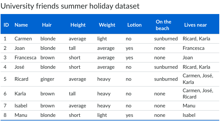
Isabel is a Attribute value Name is a Attribute Row 7 is the instance

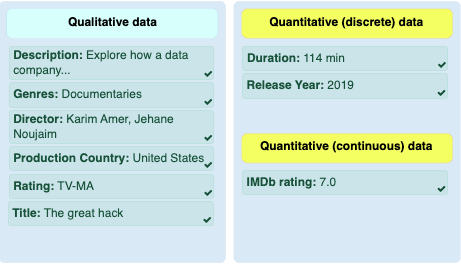
Qualitative vs Quantitative

Qualitative

less structured, non-statistical and measured using other descriptors and identifiers.

ex) polar bear is white, heavy and wild.

Quantitative

statistical and measured using hard numbers

ex) polar bear has a height of 130cm, weight 400kg and has 4 legs

Discrete quantitative

fixed, round numbers that are countable

ex) number of legs of a bear, number of times a person commutes for a job in a week

Continuous quantitative

measured over time intervals, no set fixed numbers

ex) weight of a bear, temperature of the room

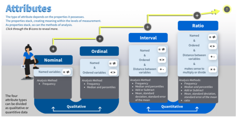
Attribute types

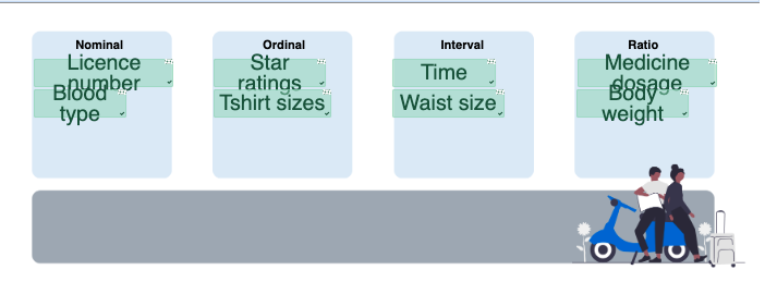
Categorical (Nominal)

Qualitative

Name! distinct symbols and values, act as labels or names. Cannot be arranged in any particular order.

Numbers can be used to program nominal variables, though basic stat calculations like mean median or standard deviation would be useless in this type.

ex) attribute Hair, values:{‘blonde’, ‘brown’, ‘ginger’}
postcodes - its a number but are just labels
industry codes, field of research codes

equality test can be performed

ex) if Hair = blonde and Lotion = no, then OnTheBeach = sunburned

Operations:

Mode, entropy, contingency, correlation, Chi squared test

Ordinal

values of an ordinal attribute provide enough information to order objects (<,>).

The categories are ordered and the transitivity remains within the process except that the distance between values is not defined

In ordinal data, addition and subtraction don’t make sense:

It’s possible to take the mean value of a binary attribute, and some methods use it to make probability distributions of the state of the outputs.

Operations: Median, percentiles, rank correlation, run tests, sign tests

Interval

Interval attributes are not only ordered but also measured in fixed and equal units. There is order, and the difference between two values is meaningful.

ex)

height, if measured as a quantity, e.g. in centimetres
weight, if measured as a quantity, e.g. in kilograms.

the difference between two values makes sense

ex)

• time in a 12-hour format is a rotational measure that keeps restarting periodicity
• the numbers are on an interval scale as the distance between them is measurable and comparable
• e.g. the difference between 5 minutes and 10 minutes is the same as 15 minutes and 20 minutes.

Operations:

differences between values are meaningful, i.e. a unit of measurement exists, because of this, it makes sense to add or subtract (+ -) when working with this data.

Mean, standard deviation, Pearson’s correlation, T and F tests

Ratio

both differences and ratios are meaningful.

Ratio attributes are ones where the measurement scheme defines a zero point (the origin of the scale). A ratio variable has all the properties of an interval variable, and also has a clear definition of zero

When the variable equals zero, there is none of that variable. Ratio quantities are treated as real numbers and all the mathematical operations including addition, subtraction, multiplication and division can be performed (…x, ÷).

Some examples:

age, values in years income, values in thousands of dollars. Temperature in kelvin monetary quantities, counts, age, mass, length, electrical current

Operations: Geometric Mean Harmonic mean, Percent variation

Each level of measurement classifies the description of the values assigned to the variables. Nominal gives the least amount of information, ordinal gives the next highest amount of information, and interval and ratio give the most information. Explore the interactive below to compare the different attribute types.

Categorising Datasets

Unstructured Data

expressed in natural language and no specific structure and domain types are defined, such as documents and sounds.

Structured Data

has an associated fixed data structure. Relational tables are typical structured data. Structured data is more manageable than other types of data.

Structured data follows a data model, has a well-outlined structure, follows a consistent order and can be easily accessed and used by a person or a computer program.

Dimensionality

A data analyst might be interested in the number of attributes for each record. Datasets with higher numbers of attributes have more dimensions. It’s often challenging to work with high dimensional data, which leads to the ‘curse of dimensionality’ and its related issues.

The curse of dimensionality refers to the classification, organisation, and analysis of high-dimensional data in high-dimensional space.

It seems obvious that more dimensions of data would help with learning, but sometimes the increase in the number of dimensions requires much more data to understand the underlying space and make good predictions.

Real life data is usually in a lower dimensional manifold - so many dimensions can be either ignored or the dimensionality can be reduced.

There is local smoothness, small changes in input values give small changes in target values, so we can do local interpolation to make predictions.

Sparsity

A dataset termed spare data or having the property of sparsity, which contains many zeros values for most of the attributes.

Resolution

The patterns depend on the scale or level of resolution. For instance, for sales figures and stocks, depending on the scale you might see daily, weekly, monthly, or yearly trends and patterns.

Semi-structured Data

format is not fixed and has some degree of flexibility. The mark-up language XML is an example of semi-structured data.

A category which is the mix of structured and unstructured data is known as semi-structured. It does not exist in relational databases but it has some organisational properties, i.e. metadata, which make it a bit easier to analyse.

One example could be an image which is unstructured by itself. However, that image/photo may have the date and time stamp if captured through a smart device, and after storage one can tag a photo that would provide a structure, e.g. ‘car’ or ‘train’. In most cases, the unstructured data is classified as semi-structured data due to its classifying characteristics.

ex) emails, text data, image, video and sound, zipped files, web pages.

Other ways to categorize

Record Data

it is assumed that the data is a collection of records (data objects) and each record consists of a fixed set of attributes.

There would be the same number of attributes for each instance

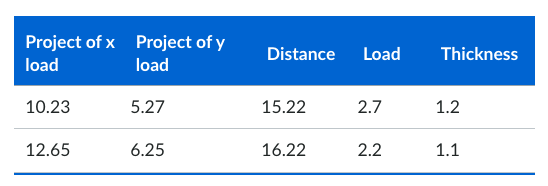
Data Matrix

In the case of a data object where each record has the exact same set of numeric attributes, they can be thought of as points (vectors) in a multidimensional space, where each dimension denotes a distinct attribute describing the object,

Such a dataset can be represented by a x * y matrix, with x rows, one for each object, and y columns, one for each attribute. Standard matrix operations can be used to transmute and control the data. Hence, the data matrix is the standard data format for most statistical data.

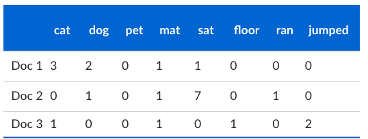
Document data

This is a special type of data matrix where the attributes are of the same type and are asymmetric. We can transfer a text document to this format for analysis. The value of each component is the number of times the corresponding term occurs in the document.

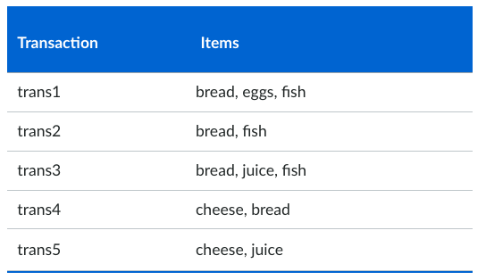
Transaction Data

This is a special type of record data. Each record (transaction) involves a set of items, as shown in table to the right. For example, a set of products bought by a customer during one shopping trip are the transaction.

Transaction data is a group of sets of items, but it can be viewed as a set of records whose fields are asymmetric attributes. Most often, the attributes are binary, indicating whether or not an item was purchased.

Graph Data

Graph data is a data structure that consists of nodes and arrows or lines. Two nodes are connected by lines in the graph. For instance, the structure of a social media network can be represented by a graph, where the nodes are the users and the links between nodes are communication devices.

Graphs form a complex and expressive data type and certain methods are required for representing graphs in databases, for manipulating and querying them. An example of the usage of graph data is Facebook or LinkedIn

WWW

provides users with access to a massive collection of documents that are interlinked through hypertext or hypermedia links, or in other terms hyperlinks.

Hyperlinks are the form of electronic connections that link related pieces of information to allow a user easy access to documents. These connections enable users to choose a word or phrase from text and thereby access other documents that contain additional information about that word or phrase.

Molecular structures

SMILES is a very powerful way of expressing structures and allows the representation of various types of atoms, bonds, rings and even complex concepts,

Ordered Data

known as sequence data, which consists of a dataset that is a sequence of individual entities, such as a sequence of words or letters. There are positions in an ordered sequence in this data type, like those found in biological sequence data i.e. genomes, proteins.

Spatial data

The geographic information of Earth and its features make spatial data. Also known as geospatial data or geographic information, spatial data is the form of data that classifies the geographic location of features and boundaries on Earth, for instance, natural or constructed features, oceans and so forth.

Spatial data can be recurrently accessed, manipulated and analysed through Geographic Information Systems (GIS). Moreover, spatial data can exist in diverse formats and includes more than just location specific information.

Temporal Data

representation of a state in time, for instance, the spread of Spanish flu in 1918, or total solar irradiation in Sydney on May 1, 2019. Temporal data is gathered to analyse weather patterns and other climate variables, observe traffic conditions and study demographic trends, etc.

The method for collecting temporal data varies from manual data entry to data acquisition through monitoring sensors, and it can also be generated through simulation models. Temporal data must be visualised for the identification of patterns or trends that emerge in the data over time, for example, tracking hurricane paths and other meteorological events, mapping the progression of wildfires or floods, or visualising variations in the occurrence of viruses over time.

Sequential Data

row of item sets and each item in the same item set has the same timestamp. Sequences are formed chronologically, i.e. a sequence of successive goods bought by customers from a company, sequence of types of activity carried out by teams in an organisation, a sequence of web page usage and a sequence of career and family life trajectories.

In some cases, sequences are timeless, e.g. sequences of proteins or nucleotides or sequences of characters and/or words in texts. Also, it varies from discipline to discipline and can depend upon the subjective needs of a project.

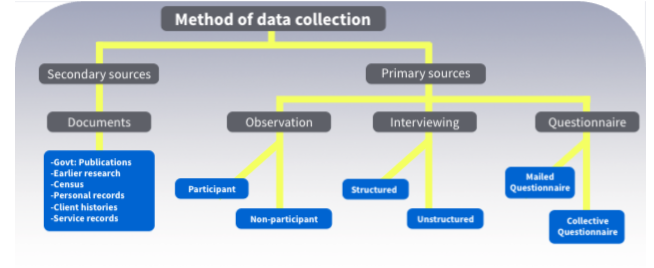
Data collection

Data collection is a process of acquiring information from all the relevant sources for finding solutions or answers to the research problem. It is the process of testing the hypothesis and evaluating the outcomes.

Quality

quality of data plays a vital role to drive the revenue of a business. On the other hand, poor quality data reduces the revenue of the business or can compromises the effectiveness of an operation or business plan.

There are several issues that can compromise data quality, which are often seen in real-world data. A range of questions can be raised to understand data quality issues:

• What are the kinds of data quality problems?
• How can we detect them (for example, in big datasets)?
• What can we do about them (for example, automatically)?

Missing values

There might be missing values for some of the attributes in the dataset. This could be because the data was not collected (e.g. age), or some attributes may not be applicable in all cases (e.g. annual income for children).

Other causes of missing values include data entry errors, changes in software design, merging different data sources with different attributes (e.g. addresses). This problem can be handled by eliminating attributes with the missing values, but we should be careful in choosing these attributes as some of them may be critical to the analysis.

Empty values

In data analytics, it’s crucial to differentiate between missing and empty values. Unlike missing values, an empty value is the one that has no actual value, whereas a missing value has an actual value but it is missing somehow.

For example, a shop sells ham sandwiches with either Swiss or tasty cheese. The shop keeps records of customer purchases to predict customer preferences and to control the inventory. The data attributes include: Gender = {‘M’, ‘F’}, Cheese type = {‘Swiss’, ‘tasty’}. Suppose a customer requests a sandwich with no cheese, and the cashier forgets to enter the customer gender. Therefore, the transaction would eventually end up with no values for both fields ‘gender’ and ‘cheese type’, but the value for gender is missing, while the value for cheese is empty but not missing.

Noise

Noise is the modification of actual values. Noise is the random component of a measurement error and it involves either the distortion of the value or the addition of objects that are unnecessary.

For example, distortion of the voice while talking on poor phone lines. The figure below demonstrates a time series before and after disruption by some random noise.

Outliers

Outliers are a single or very low frequency occurrence of a value of an attribute that is far from the bulk of attribute values, as shown in the figure below. It is essential to distinguish between noise and outliers. Outliers can be legitimate data objects or values. Thus, unlike noise, outliers may sometimes be of interest.

Duplicate data

Datasets might include data objects that are almost imitations of others. To mitigate these duplications, a couple of issues must be addressed.

First, if there are two objects that actually represent a single object, then the values of corresponding attributes may vary, and these uneven values must be resolved. Second, caution is essential to avoid accidentally combining data objects that are alike, but not duplicates. Examples include the same person with multiple email addresses or people who changed their name when they married.

Inconsistent formats

Data inconsistency occurs when the same set of data appears in multiple tables from different inputs. For instance, consider a phone number, where both a city and country code are listed, but the specified city code is not contained in that number.